How I Iterate and Plan for Successful Outcomes

The first thing the pipeline told me was that my data assumption was wrong. I had designed a retrieval system around the idea that every contact record had a primary email field. They did not. Forty-three percent of the records in that CRM had the email buried in a notes field as free text. The embedding model indexed the field I told it to index. The retrieval returned nothing useful. That was day one, and it rewrote the entire architecture before I had written a single chunk strategy.

In my opinion, every plan I write is a hypothesis. The data is the test. I validate step one before designing step two, not because I lack discipline, but because the data always knows something I do not. The projects that collapse at month four are the ones where someone wrote a 30-page spec against an assumed data shape and never checked that shape against reality. By the time they found out it was wrong, they had built the wrong thing at scale.

This is the process I actually use. It is not elegant. It involves discovering that your assumptions are wrong at every step. That is the point.

Why the Spec Always Breaks at the Data Layer

The standard approach is to architect before auditing. Design the retrieval pipeline, pick the embedding model, choose the chunking strategy, wire the generation layer. All of this happens against an assumed data shape. The data shape is wrong. It is always wrong in some way that matters.

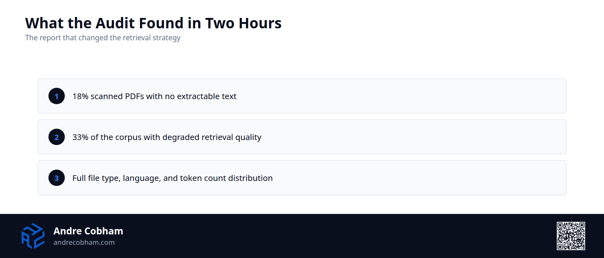
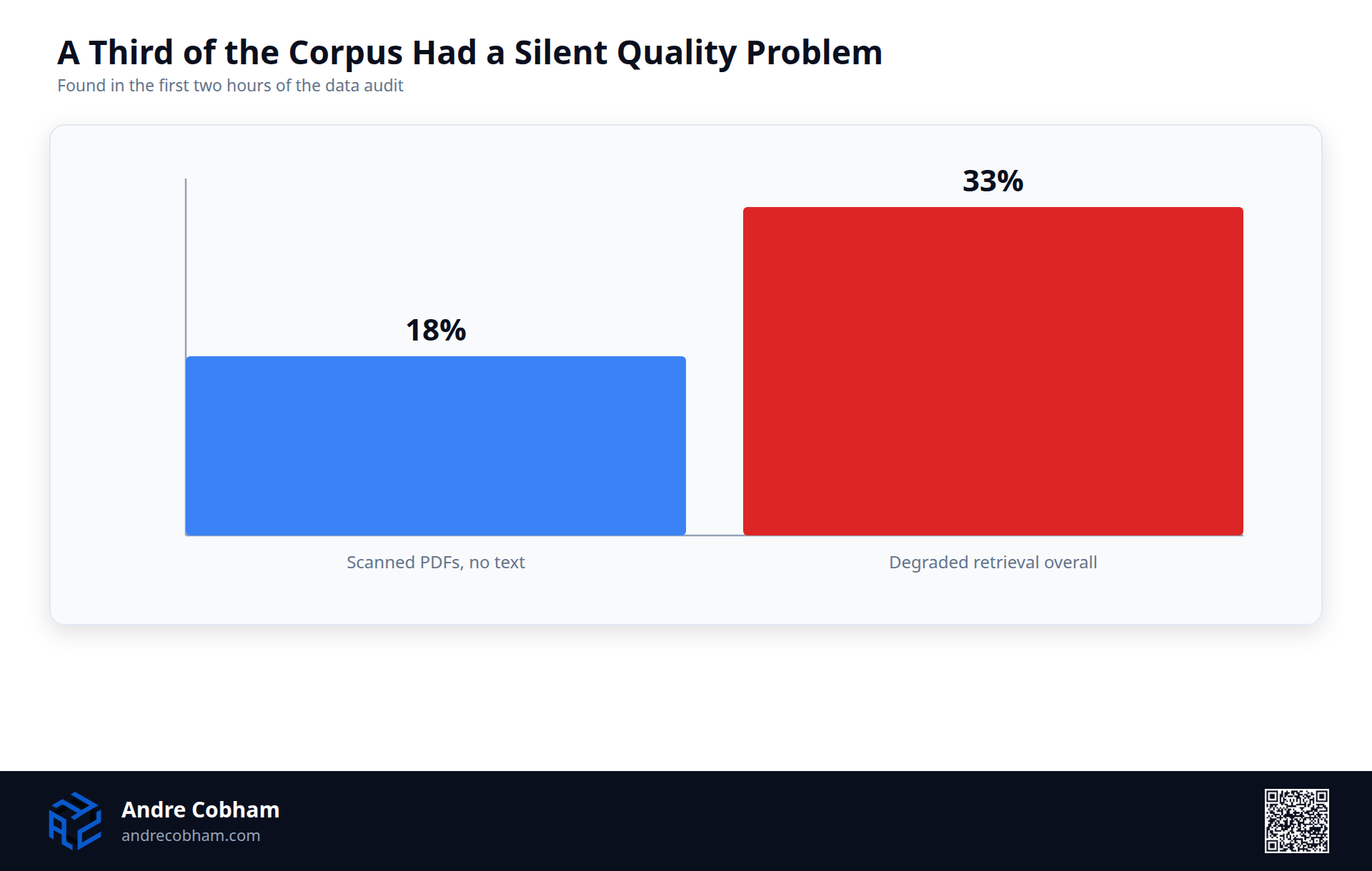
The pipeline ran on a 52,000-document corpus pulled from Google Drive. The assumption was that documents were mostly English-language proposals and reports, clean prose, consistent structure, good candidates for recursive character splitting before embedding with OpenAI text-embedding-3-large. The data audit found 18% were scanned PDFs with no extractable text. Nine percent were spreadsheets. Six percent were in Spanish. My chunking strategy, built for English prose, performed poorly on all three categories. That is 33% of the corpus with degraded retrieval quality, and I found it in the first two hours of the data audit. If I had found it at week six, after building the retrieval layer, the vector store, and the generation wrapper, the fix would have cost three weeks, not two hours.

When you discover schema problems after building against them, you pay twice, once to understand the real shape, once to redo the work that assumed the wrong shape. The data audit is not a preliminary step. It is step one, and everything else waits for it.

How I Structure a Pipeline Build

Five steps. Sequential by design. You do not skip forward.

Step 1: Data audit with real data before any model decisions. Profile the corpus. For that 52,000-document set, I wrote a Python script against the Drive API to pull file metadata, detect MIME types, sample content, and flag anything that was not plain text or structured prose. The audit output was a JSON report: file type distribution, language distribution, mean token count per document, percentage of documents below 200 tokens (too short to chunk meaningfully), percentage above 8,000 tokens (will exceed context window without aggressive chunking). No model decision gets made until this report exists.

Step 2: Define one pipeline step with a measurable pass/fail condition. Not a phase. Not a milestone. One step. For a retrieval layer, that looks like: retrieval precision@5 above 0.75 on a 50-query test set drawn from real user queries. If I cannot write the acceptance criterion as a number, the step is not defined well enough to build.

Step 3: Run it with real data and measure the output. Not synthetic data. Not hand-picked examples. Real data, full pipeline, against the eval set. I use LangChain for orchestration during the build phase because it makes it easy to swap the retriever or the embedding model without rewriting the evaluation harness. The eval set runs the same way every time.

Step 4: Validate the measurement before designing step two. If precision@5 is 0.58 and the threshold is 0.75, step two does not start. I debug the retrieval layer, check chunk sizes, check embedding quality by inspecting nearest neighbors in Pinecone or Weaviate for a sample of queries, check whether the query encoder is aligned with the document encoder. Step two is designed from what step one actually achieved, not from what I expected it to achieve.

Step 5: Each completed step revises the assumption behind the next. By step four or five, I am building against confirmed data shapes, confirmed retrieval behavior, confirmed latency profiles. The uncertainty surface is narrow. That is what makes late-stage builds fast.

The key discipline across all five steps is that the acceptance criterion is a number, not a feeling. Retrieval precision. Hallucination rate on a held-out eval set using Ragas or a custom faithfulness scorer. Latency at p95 under a realistic concurrency load. If you cannot measure it, you cannot call it done.

What This Looks Like Across a Multi-System RAG Build

This approach produced a four-source RAG pipeline for a professional services firm. Sources were a CRM (HubSpot, contact records, deal history, notes), Google Drive (proposals, SOWs, reports), email threads (IMAP extraction from Gmail), and an internal Notion wiki. The goal was a query interface that could answer questions about client history and deal context from all four sources simultaneously.

The spec written before step one had one preprocessing pipeline. After step one, there were four.

The CRM data had three years of import history, which meant three different field naming conventions and two different approaches to storing contact notes. The HubSpot REST API returned records that looked consistent in the UI but had inconsistent schema in the raw JSON. Before any of that data could be embedded with text-embedding-3-small, it needed entity extraction, pulling company names, deal values, and dates out of free-text note fields and attaching them as metadata on the chunk so filters would work downstream.

The email threads needed deduplication and thread reconstruction. A thread with 12 replies exists in the IMAP export as 12 separate messages, each containing the full prior context quoted at the bottom. Without thread reconstruction, the embedding index would have 12 nearly-identical chunks per thread, and retrieval would return them all, collapsing the context window before reaching a useful result. I wrote a threading script using the In-Reply-To and References headers before any emails touched the vector store.

The Notion wiki needed a staleness filter. Pages not updated in 18 months had factually outdated content, old pricing, departed team members, discontinued services. Using them as retrieval context would inject wrong answers confidently. The filter was simple: pull the last_edited_time from the Notion API and exclude pages older than 18 months from the index. That one filter changed the character of retrieved context meaningfully.

None of these preprocessing requirements existed in the original spec. All of them were discovered in the first pass through the data from each source.

When the Retrieval Starts Lying to You

I run a cross-session memory database called hop.db that stores observations, decisions, and outcomes from every AI session I run. It is a SQLite database with an FTS5 full-text search index over roughly 82,000 rows. The idea is straightforward: anything that would be useful to remember across sessions gets written in. At the start of a session, relevant facts surface automatically. The system compounds across time.

About four months after the initial build, the retrieval was degrading. Queries that should surface the five most relevant rows were returning results that were six or seven rows off from what I wanted, or returning the right category of fact but the wrong specific instance. The problem was not immediately obvious because the results were not wrong in a loud way. They were wrong in a quiet way, plausible-looking facts from the right domain but not the ones the query was actually asking for.

In my opinion, the root cause was FTS5 degradation under corpus growth. SQLite's FTS5 index uses a BM25-based ranking that works well on smaller corpora but drifts as the index grows and term frequencies shift. At 80,000 rows, the IDF (inverse document frequency) weights had changed enough that common terms in the most recent additions were pulling results toward recently-written rows regardless of semantic relevance. The query "CIFS mount stall handling" was surfacing rows about mount configuration from the past two weeks rather than the specific diagnosis I wrote three months ago when I actually solved the problem.

The Semantic Summary Fix

The structural fix was adding a semantic summary column to the hop.db schema. One sentence per row, written at insert time, describing what the row contains in terms a retrieval query would use. The summary is not a restatement of the content. It is a distillation of the retrieval signal: what is this row about, phrased the way someone would ask for it.

The difference in practice looks like this. A raw row might say: "Ran the SYCL build with MKL flags disabled, got 14.2 t/s on Qwen3-8B. Tried again with AVX512 forced, dropped to 11.8 t/s. The MKL path is faster on this chip." The semantic summary for that row: "Qwen3-8B SYCL inference throughput comparison, MKL vs AVX512 on local hardware." When a query comes in asking about Qwen3-8B inference performance, the summary matches more cleanly than the raw content, which buries the relevant terms in a narrative of observations.

The retrieval query now runs against the summary column first using FTS5, then scores the top candidates with vector similarity on the full content. The hybrid approach handles both keyword specificity (which FTS5 does well) and semantic intent (which pure keyword search misses). Precision on the same test queries I used to diagnose the degradation went from landing the right row in the top 5 about 60% of the time to landing it in the top 3 about 87% of the time.

Running the Enrichment Pipeline at 82,000 Rows Without a Cloud Bill

Adding summaries to 82,000 existing rows required a local enrichment run. Sending each row to a cloud API would have cost somewhere between $40 and $80 depending on the model, which is not a prohibitive number, but more importantly it would have sent 82,000 rows of operational notes and system observations to an external service. That is data I do not want leaving the machine.

Qwen3-8B ran locally via Ollama on a workstation with an integrated Intel Arc GPU. The model runs at roughly 14 tokens per second on that hardware using the SYCL backend. Each summary generation averaged about 40 tokens of output. At 14 tokens per second, that is roughly 3 seconds per row, or about 68 hours of continuous inference for the full 82,000-row backfill. The batch ran in 1,000-row increments overnight over five nights, checkpointing progress to a separate table so restarts did not repeat completed rows.

The prompt was kept simple: "In one sentence, describe what this observation is about and what it would be useful for finding. Be specific about tools, systems, and outcomes mentioned." Simple prompts on a smaller model at this task outperformed elaborate prompts in my tests. The model is good enough at one-sentence summarization that you do not need to engineer around it. The constraint is getting it to stay to one sentence rather than expanding into a paragraph, which an explicit instruction handles cleanly.

The Function Planner Layer

The enriched hop.db feeds a function-planning layer that maps intent to available tools. I have 503 scripts in a toolbox directory, each registered in a separate SQLite database with a name, description, category, and RL-scored weight. The weight starts at 1.0 when a script is registered and updates after each use based on whether the outcome was successful.

The scoring is simple. A run completes and a result gets written: success, partial, or fail. Success increments the weight by 0.1. Partial holds it flat. Fail decrements by 0.15. After 30 uses, a script with a weight above 1.3 is reliably useful for the tasks it gets dispatched on. A script below 0.7 surfaces a warning. Below 0.5 it stops appearing in recommendations. The system prunes itself without requiring manual curation.

The function planner at session start does three lookups: semantic search over hop.db for context relevant to the current task, keyword search over the toolbox database for scripts matching the task keywords, and a cross-reference to check whether any of the returned toolbox scripts have been used on similar hop.db entries before. The intersection of those three results is the recommendation. It is not sophisticated reasoning. It is structured lookup with weighted ranking. But it means that on the 40th time I am doing something similar to something I have done before, I start with the tools that worked, not a blank page.

When the Agent Is the One Iterating

Agentic systems change what iteration means. In a standard pipeline, I am the one who finds the wrong assumption and revises the spec. In an agentic system, the model calls tools and the tool returns are what change the plan. The agent is iterating. It is doing it at runtime, not in a planning meeting.

A customer research agent built for a client had three tools: search_crm(query), read_document(doc_id), and query_knowledge_base(query). The planner prompt told the agent to start with search_crm to pull account history before reading any documents. On the first real run in production, search_crm returned zero results. Not because the account did not exist, because the CRM field name in production was account_name and the staging environment had used company_name. The agent's tool call returned empty, and the plan had to branch at step one based on what the environment actually contained.

I had written the tool calling logic to fail loudly on empty returns. The agent received the error, logged it, and fell back to query_knowledge_base with the account identifier instead. That fallback was in the system prompt as an explicit recovery path, not because I anticipated that specific failure, but because I had built the agent to recover from unexpected tool returns rather than halt on them. The plan at dispatch time was not the plan at completion. The agent had revised it based on what the functions returned.

Building agentic systems for this requires designing recovery paths into the prompts, not just designing the happy path and hoping the environment matches the spec. Every tool call is a hypothesis about what the environment contains. The tool return is the test.

What Breaks This System

From my perspective, the hop.db pipeline has three failure modes I have hit in production. CIFS mount stalls are the most disruptive. The database lives on a network share mounted via CIFS, and when the mount stalls, SQLite WAL (write-ahead log) files can accumulate without being checkpointed. If the stall happens mid-write, you get a locked database that requires manual WAL recovery before any reads succeed. The fix was adding a mount health check before every hop.db write, with a 30-second timeout and automatic remount on failure. The check adds latency but the alternative is corrupted state that takes 20 minutes to recover from.

SQLite WAL conflicts are the second failure mode. When multiple agent sessions write to hop.db concurrently, WAL checkpoint conflicts produce "database is locked" errors. SQLite supports concurrent reads but serializes writes, and with several agent processes writing summaries simultaneously the queue can back up. The fix was a write queue with a single writer process and a socket-based interface for agent processes to submit writes without touching the database directly. The queue is overkill for most workloads but the failure mode it prevents is data loss, which made it worth building.

Context window limits at 300,000 tokens are the third constraint. The hop.db retrieval returns 20 rows by default. At the start of a complex session, those 20 rows plus the system prompt plus the task description can push toward the context limit before any real work starts. The mitigation is a token budget for retrieved context, truncating the hop.db results to fit within a fixed allocation rather than returning a fixed row count. The right number depends on what else is in the context, so this is calculated dynamically rather than hardcoded.

Measuring Before You Call It Done

Retrieval pipelines feel like they are working before they are actually working. The trap is testing with five hand-picked queries that all retrieve well, calling the retrieval layer done, and then hitting 500 query patterns in production where precision collapses on the long tail. The five queries you picked were the easy ones. They always are.

Before I declare any retrieval step complete, I run four checks. A 50-query eval set built from real user queries or realistic variants, not queries I made up, queries that came from the team that will actually use the system. Precision@5 against that set: are the top five retrieved chunks actually relevant to the query. A faithfulness check on a 20-question sample using the generated answers: does the answer stay inside what was retrieved or does the model go outside the context. Latency at p95 under a realistic concurrency load, not a single-threaded timing test, but 10 concurrent requests to see where the embedding step or the vector store query starts to buckle.

If any of those fail the threshold, step two does not start. This is the discipline that separates pipelines that work at scale from ones that worked in the demo.

What I Would Build Differently If Starting Over

The hop.db architecture I have now works, but it carries the weight of decisions made before I understood the problem well. If I were starting the cross-session memory system from scratch today, I would design the semantic summary in from the beginning rather than retrofitting it at 82,000 rows. The enrichment backfill took five nights of local inference. If every row had been summarized at write time, that cost would have been distributed across months instead of paid all at once.

I would also separate the write path from the read path from the start. A single SQLite file serving both concurrent writes and real-time reads is workable but fragile under load. The write queue I added later is the right architecture, but adding it to an existing system required careful migration to avoid losing in-flight data. Building it in from the beginning would have been a two-hour design decision instead of a half-day migration.

The RL scoring on toolbox scripts I would keep exactly as is. It is the simplest possible implementation of something that compounds over time: a weight that reflects usage history, updated automatically, pruning the toolbox toward what actually works without any manual intervention. The discipline that makes it valuable is writing outcomes back consistently. The system is only as good as the completeness of the feedback it receives.

Iteration Is Not Undisciplined

The objection I hear most often is that iterative approaches produce scope creep and lack accountability. The critique is valid when iteration means starting without a definition of success. That is not what I am describing. Every step has an explicit acceptance criterion. You either hit the number or you do not. There is no ambiguity about whether the step is done.

A 30-page spec has one decision point, the moment you sign off on it, when you know the least about the actual system. An iterative pipeline build has a decision point after every step, when you know the most you have ever known about the system up to that moment. More decision points means more chances to catch the wrong assumption before it is embedded in the architecture. The spec is not the discipline. The measurement is.

If you are starting a pipeline build this week, the most useful thing you can do today is define step one and its acceptance criterion. Not the full architecture. One retrieval or preprocessing step, one measurable output, one pass/fail number. Run it against real data. See what it tells you. Design step two from what you now know.

The plan is a hypothesis. The data is the test. Everything else follows from what the data returns.